How to Find the Trading Strategy That Beats the Market in Python
Find out which of your trading strategies beats buy and hold, scored only on days the tuning never saw. One Python command runs the walk-forward test with fees and slippage, and on the practice stock breakout-v1 made +37.0% against +21.6% for the benchmark.
>This covers the walk-forward scorecard. The AI Trading Agent Alpha Swarm Team adds the five agents that trade the winning strategies, the broker connection and the rules for retiring a strategy that stops winning.
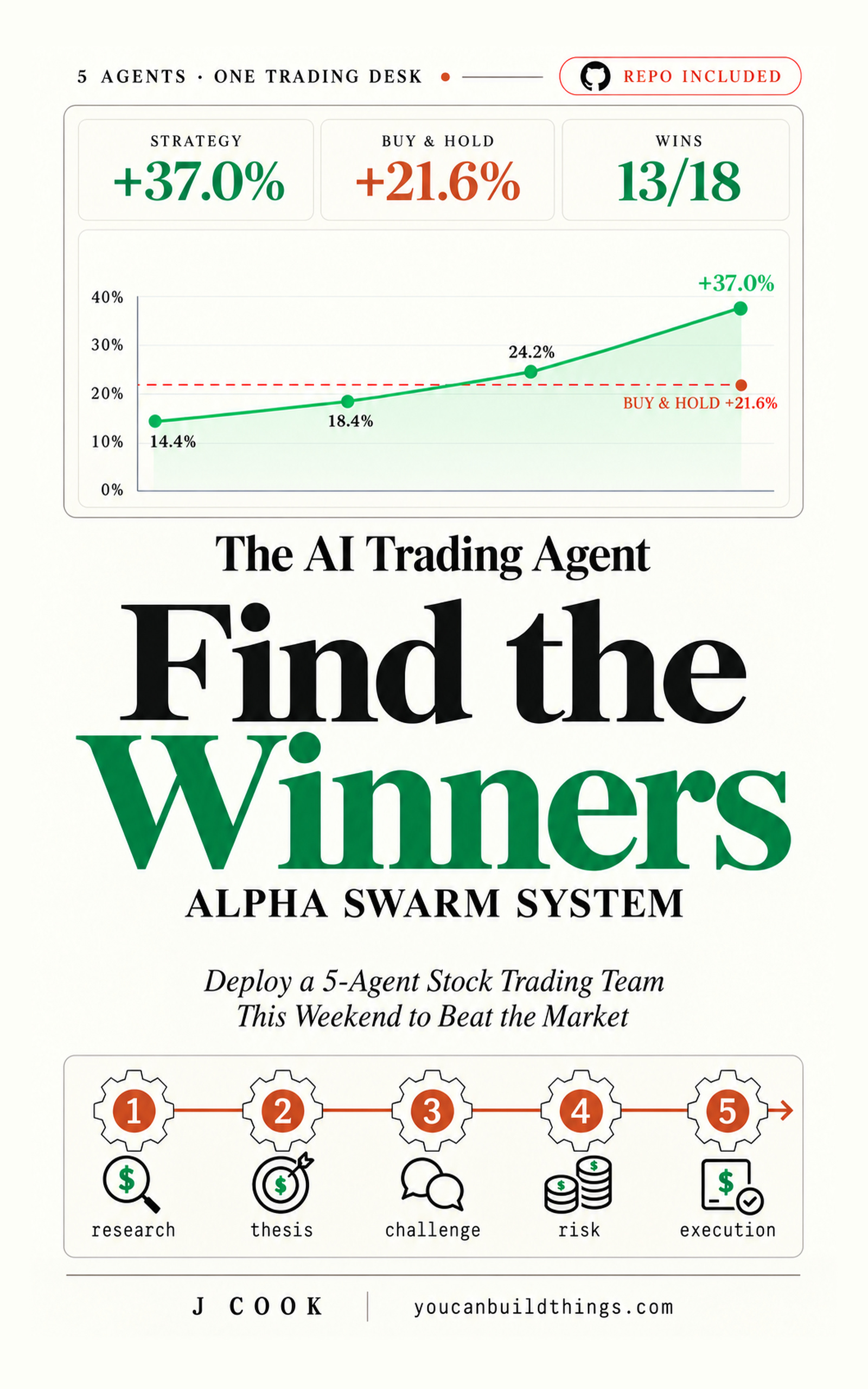
The AI Trading Agent Alpha Swarm Team
Deploy a 5-Agent Stock Trading Team This Weekend to Beat the Market and Find Winners
Hello builders,
By Sunday afternoon you can know which of your trading strategies beats the market, measured on days the tuning never saw. Most people find out in public, in a Reddit thread where a reply with 11 upvotes opens with one word in capitals: “FAKE. I backtested this strategy and it is nowhere near what the guy is saying.” The tool we use here is the walk forward backtest Python script from my book, and every run ends in a column called beat? that says YES or no.
Another reply with 15 upvotes said “Sharpe ratio is about 0.6,” and a third warned that 5.93% over three months “could be purely luck.” Was it tested on data it hadn’t seen, and could the whole result be luck? The scorecard below prints the trade count, the luck number, the cost and the result on unseen days for every strategy you own.
Tune on 252, score on 126
We take 252 trading days, about a year, try each setting of a strategy on those days and keep the best one. Then we run that setting on the next 126 days, which it has never seen, and write down only what happened there. Slide everything forward 126 days and do it again.
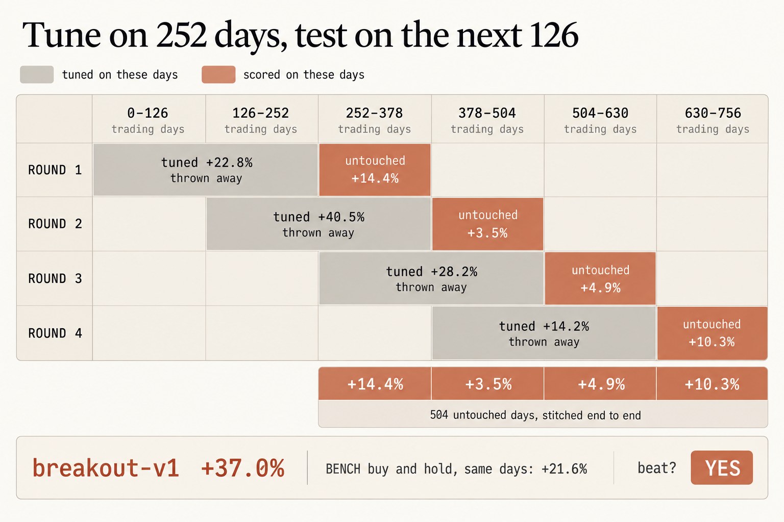
We throw the tuned days away, because the setting was picked for doing well on them. On 756 days of practice data that leaves four rounds. Breakout-v1 made +22.8% on its first tuning window and +14.4% on the 126 days after it. Then +40.5% tuned and +3.5% untouched, +28.2% and +4.9%, and +14.2% and +10.3%. Stitch the four untouched windows end to end and you get 504 days the tuning never touched: +37.0% for breakout-v1, against +21.6% for buying the benchmark and holding it over the same days.
This test runs on the strategy rules alone, with the four model seats switched off, and a post on X gave the reason in one line: “It read those years’ news in training, so ‘predicting’ them is partly recall.” I agree with that post, and it is why our past-markets test leaves the models out entirely.
One command, three strategies
You need Python 3.12 or newer and no account. DEMO is a made-up stock whose prices come from a formula, and I built it so the three setups would land in three different places, so your numbers will match mine exactly.
git clone https://github.com/regardo911/alpha-swarm.git
cd alpha-swarm
python3 -m venv .venv
source .venv/bin/activate
python make_fixture.py
python walkforward.py DEMO
DEMO: untouched days 2021-12-22 to 2023-11-27
BENCH buy and hold, same days: +21.6%
strategy net trades wins maxDD sharpe t cost$ beat?
breakout-v1 +37.0% 18 13 8.2% 1.43 2.0 21.65 YES
pullback-v1 +8.8% 12 8 10.6% 0.48 0.7 12.46 no
bounce-v1 -6.5% 17 7 27.2% -0.24 -0.3 17.67 no
breakout-v1: 20 signals, 2 never filled
pullback-v1: 14 signals, 2 never filled
bounce-v1: 18 signals, 1 never filled
saved cards/DEMO.jsonRead the second line first, because +21.6% is the bar every row has to clear. Breakout made 37.0% after costs over 18 trades with 13 wins and cleared it. Pullback made 8.8% and finished under the benchmark, and bounce lost 6.5% after sitting 27.2% below its own high at the worst point. The t column is the luck meter, and William Sharpe gave the link himself:
The t-statistic will equal the Sharpe Ratio times the square root of T (the number of returns used for the calculation).
(William F. Sharpe, “The Sharpe Ratio”)
Breakout’s t is 2.0 over 504 days and bounce’s is -0.3, and I read the bigger number as the result that’s harder to explain by chance.
Catch the overfit yourself
Add a strategy name, as in python walkforward.py DEMO bounce-v1, and the test prints each round’s tuned result next to its untouched one.
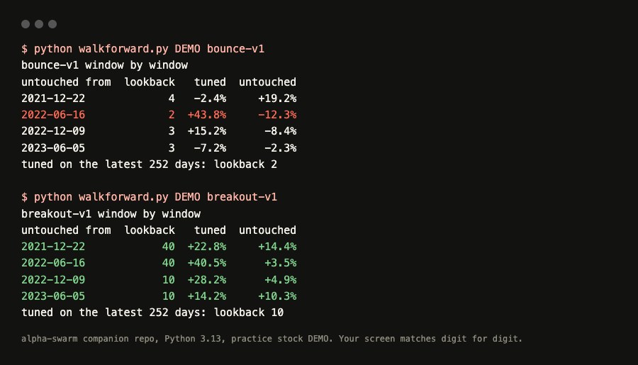
Look at the second row for bounce, where a two-day lookback made 43.8% on the days it was tuned on and then lost 12.3% on the next 126 days. Stopping at the tuning window would have meant posting a 43.8% screenshot for a setting that went on to lose money. Breakout’s untouched results came in lower than its tuned ones in every row and stayed positive in all four, which is about as good as I’d expect a real strategy to look on unseen days.
Every trade in our test pays, too. The script takes 5 hundredths of a percent off each fill for slippage, a cent per buy and two cents per sell, so the breakout result above has already paid $21.65 in slippage and fees on a $1,000 account. For comparison, here is the default slippage model in QuantConnect’s LEAN engine, a widely used open-source backtester, on its current master branch:
// Common/Orders/Slippage/NullSlippageModel.cs
/// Null slippage model, which provider no slippage
public sealed class NullSlippageModel : ISlippageModel
{
    public decimal GetSlippageApproximation(Security asset, Order order)
    {
        return 0;
    }
}Now run it on a stock you actually watch, against the real market. Install the broker package with python -m pip install alpaca-py==0.44.0, put your Alpaca keys in keys.env, and python live.py XYZ SPY downloads six years of daily prices for your symbol and SPY, and python walkforward.py XYZ prints the same table with SPY as the bar. The stock needs about a year and a half of history before it has an untouched window. Whatever it prints is your strategy measured against the real market on days it never saw, and the rows that say YES are the strategies that earn a trade on Monday.
Now go build something this weekend!
John Cook