Monte Carlo Backtesting for Trading Strategies

Summary:

1. Build a Python backtester that shuffles trade returns 1,000 times and simulates equity curves.
2. Use the 5th percentile as a binary go/no-go decision: positive means real edge, negative means no edge.
3. Detect overfitting with an in-sample vs. out-of-sample split before going live.
4. Copy-paste framework with Sharpe ratio, profit factor, fan chart, and JSON report.

My screener bot ran for three weeks. Twelve out of sixteen trades profitable. 75% win rate. I was already picking out furniture for the new apartment.

Then I ran the backtest. The 75% dropped to 52% over six months of historical data. The eye-popping results from three weeks were a hot streak in a bull market. If I had gone live with $10,000 based on three weeks of paper trading, I would have paid real money to learn about sample size.

Why does a single backtest lie to you?

A single backtest tells you what happened in one specific sequence. Markets went up on these days, down on those days, your strategy produced these results. But what if the big winner that carried your Q3 had happened during a drawdown? What if three losing trades clustered together instead of being spread out?

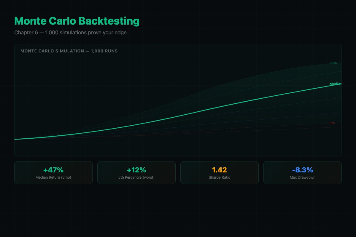
Monte Carlo simulation answers these questions by shuffling the deck. Take your trade results, randomly reorder them, simulate the equity curve. Do it 1,000 times. Each simulation produces a different equity curve. Some spectacular, some terrible, most in the middle.

The number that matters: the 5th percentile return. If it is positive, your strategy makes money even when luck is against you. If it is negative, your “profitable” strategy can lose money depending on trade ordering. That is not an edge. That is a coin flip dressed up as a system.

What does the input data need?

# Required trade list format
trades = [
    {"return_pct": 0.023, "date": "2025-01-15"},  # 2.3% gain
    {"return_pct": -0.011, "date": "2025-01-16"}, # 1.1% loss
]
# return_pct is a decimal (0.02 = 2%), NOT a percentage (2.0)
# Minimum 100 trades for meaningful Monte Carlo results
# Trades must be sorted by date (oldest first)

Getting the unit wrong (percentage vs decimal) is the #1 Monte Carlo implementation error.

import random
import numpy as np

def monte_carlo(returns, n_sims=1000, initial=100000, risk_pct=0.02):
    """Run Monte Carlo simulation on trade returns.

    returns: list of per-trade return percentages (e.g., [0.038, -0.021])
    n_sims: number of random shuffles
    initial: starting capital
    risk_pct: fraction of capital risked per trade
    """
    final_values = []
    max_drawdowns = []

    for _ in range(n_sims):
        shuffled = random.sample(returns, len(returns))
        capital = initial
        peak = capital
        max_dd = 0

        for ret in shuffled:
            pnl = capital * risk_pct * ret
            capital += pnl
            if capital > peak:
                peak = capital
            dd = (peak - capital) / peak
            if dd > max_dd:
                max_dd = dd

        final_values.append(capital)
        max_drawdowns.append(max_dd)

    return final_values, max_drawdowns

That is the core. About 20 lines. The shuffle-and-simulate loop is the entire idea behind Monte Carlo backtesting for trading.

How do you read Monte Carlo results?

Here is what real output looks like from a screener strategy with 423 trades over six months:

Strategy Statistics:
  Total Trades: 423
  Win Rate: 53.7%
  Avg Winner: 3.82%
  Avg Loser: -2.14%
  Profit Factor: 1.79
  Sharpe Ratio: 1.24

Monte Carlo Results (1,000 simulations):
  5th Percentile:  $108,400 (+8.4%)
  25th Percentile: $118,200 (+18.2%)
  Median:          $127,600 (+27.6%)
  75th Percentile: $138,100 (+38.1%)
  95th Percentile: $152,300 (+52.3%)
  Median Max Drawdown: 8.7%
  Worst Max Drawdown: 19.4%

VERDICT: EDGE CONFIRMED

The 5th percentile is positive. Even in the worst 5% of simulated trade orderings, you still made money. That is a real edge.

But the worst-case max drawdown is 19.4%. Your $100K account drops to $80,600 before recovering. If you cannot stomach that, reduce position size.

If you want to compare your Monte Carlo output against an institutional-grade benchmark, QuantConnect’s backtest report generates these metrics automatically for any strategy on their platform:

Probabilistic Sharpe Ratio (PSR), Compounding Annual Return, Maximum Drawdown, Win Rate, Profit-Loss Ratio, Alpha, Beta, Annual Std Deviation, Sharpe Ratio, Information Ratio, Treynor Ratio, and Estimated Strategy Capacity. Rolling statistics are sampled over 1, 3, 6, and 12-month windows with the top 5 drawdown periods highlighted.

PSR is the one most traders skip. It answers: what is the probability that your Sharpe ratio is real and not a sample-size artifact? A strategy with a 1.2 Sharpe and 95% PSR is a better bet than one with a 2.0 Sharpe and 60% PSR.

How do you build the full backtester with reporting?

def calculate_sharpe(returns, risk_free_rate=0.05):
    """Annualized Sharpe ratio."""
    arr = np.array(returns)
    excess = arr - (risk_free_rate / 252)
    if len(excess) == 0 or np.std(excess) == 0:
        return 0
    return np.mean(excess) / np.std(excess) * np.sqrt(252)

def generate_report(trades, final_values, max_drawdowns, initial):
    """Full backtest report from Monte Carlo results."""
    returns = [t["return"] for t in trades]
    win_rate = len([r for r in returns if r > 0]) / len(returns)
    avg_win = np.mean([r for r in returns if r > 0])
    avg_loss = np.mean([r for r in returns if r < 0])
    sharpe = calculate_sharpe(returns)
    pf = abs(avg_win / avg_loss) if avg_loss != 0 else float('inf')

    p5 = np.percentile(final_values, 5)
    p50 = np.percentile(final_values, 50)
    p95 = np.percentile(final_values, 95)

    return {
        "total_trades": len(trades),
        "win_rate": f"{win_rate:.1%}",
        "profit_factor": f"{pf:.2f}",
        "sharpe": f"{sharpe:.2f}",
        "p5": f"${p5:,.0f} ({(p5/initial-1)*100:+.1f}%)",
        "median": f"${p50:,.0f} ({(p50/initial-1)*100:+.1f}%)",
        "p95": f"${p95:,.0f} ({(p95/initial-1)*100:+.1f}%)",
        "worst_drawdown": f"{max(max_drawdowns):.1%}",
        "verdict": "EDGE CONFIRMED" if p5 > initial else "NO EDGE"
    }

The verdict is binary. 5th percentile above starting capital? Edge confirmed. Below? No edge. Do not rationalize a negative 5th percentile. The market will find the scenario where your strategy loses money, and it will use your real dollars.

How do you detect overfitting before it costs you money?

My first screener used seven parameters. It backtested to a 67% win rate and 2.3 Sharpe. Then I ran the out-of-sample test. Win rate: 44%. Sharpe: 0.2. The strategy lost money on unseen data.

Seven parameters gave me seven degrees of freedom to fit noise. I stripped it to three parameters: vol/OI threshold at 3.0, minimum premium at $200K, sweeps/blocks only. Training data: 53% win rate, 1.2 Sharpe. Out-of-sample: 51% win rate, 1.1 Sharpe. Almost identical. That is a real edge.

Here is the split test:

def check_overfitting(trades):
    """Split data to detect overfitting."""
    midpoint = len(trades) // 2
    in_sample = trades[:midpoint]
    out_sample = trades[midpoint:]

    in_wr = len([t for t in in_sample if t["return"] > 0]) / len(in_sample)
    out_wr = len([t for t in out_sample if t["return"] > 0]) / len(out_sample)

    gap = abs(in_wr - out_wr)
    status = "OK" if gap < 0.05 else "OVERFIT WARNING"

    print(f"In-sample win rate:  {in_wr:.1%}")
    print(f"Out-of-sample:       {out_wr:.1%}")
    print(f"Gap: {gap:.1%} [{status}]")
    return gap < 0.05

If the gap is under 5 percentage points, the edge is real. If removing a parameter drops your backtest results by less than 2 percentage points, remove it. Fewer parameters means less overfitting risk.

What broke the first time I backtested?

Two bugs that took a week to find.

Look-ahead bias. My filter used end-of-day volume and open interest numbers, but in real trading, those numbers accumulate throughout the day. A sweep at 10 AM does not have the full day’s volume available. Fix: use point-in-time data at the exact timestamp of each transaction.

Survivorship bias. My stock universe only included stocks still trading six months later. Stocks that got delisted or acquired were missing. This inflated results on the small-cap end. Fix: include all stocks that existed at each point in time, regardless of what happened later.

After fixing both, my backtest went from 58% win rate to 52%. Less flattering, more honest. I need the real number.

Fat tails warning: Monte Carlo shuffling assumes trade returns are independent and identically distributed. Real markets have fat tails (rare extreme moves) and regime shifts (calm to volatile). Your Monte Carlo 5th percentile is optimistic during a crisis. Add a stress test: what happens if your worst 5 trades all occur in the same week?

# Reproducible test dataset (use for validating your implementation)
import numpy as np
np.random.seed(42)
test_trades = [{"return_pct": r} for r in np.random.normal(0.002, 0.015, 200)]
# Expected: ~200 trades, mean ~0.2%, std ~1.5%
# Run Monte Carlo on this set. Your median final balance should be ~$114,900 on $100K start.

What should you actually do?

• If you have 50+ paper trades: run them through the Monte Carlo framework right now. If the 5th percentile is negative, stop trading and fix the strategy.
• If your backtest looks too good: run the overfitting split. If the gap exceeds 5%, simplify your parameters. The three-parameter version will underperform the seven-parameter version on historical data. It will outperform on live data.
• If you want continuous monitoring: re-run the backtest quarterly on the most recent 90 days. If the 5th percentile goes negative on recent data, something changed. Reduce position sizes by 50% and investigate.

bottom_line

• The 5th percentile is the only number that matters. It answers one question: does this strategy make money when luck is against me?
• Overfitting is the silent killer of trading bots. Seven-parameter strategies backtest beautifully and fail live. Three-parameter strategies backtest modestly and survive.
• Run the backtest before risking a dollar. The r/algotrading community has a word for going live without backtesting: gambling.