Cointegration Pairs Trading Python: Z-Score and Hedge Ratio
Cointegration pairs trading in Python with statsmodels: Engle-Granger test, Z-score entries at ±2.0, hedge-ratio sizing, 20-day time-stop, VIX regime filter.
>This is one strategy of seven. Use Claude to Build 7 AI Trading Bots ships the pairs bot, a flow bot, a funding-rate arb bot, and the multi-bot allocator that runs them together without chaos.
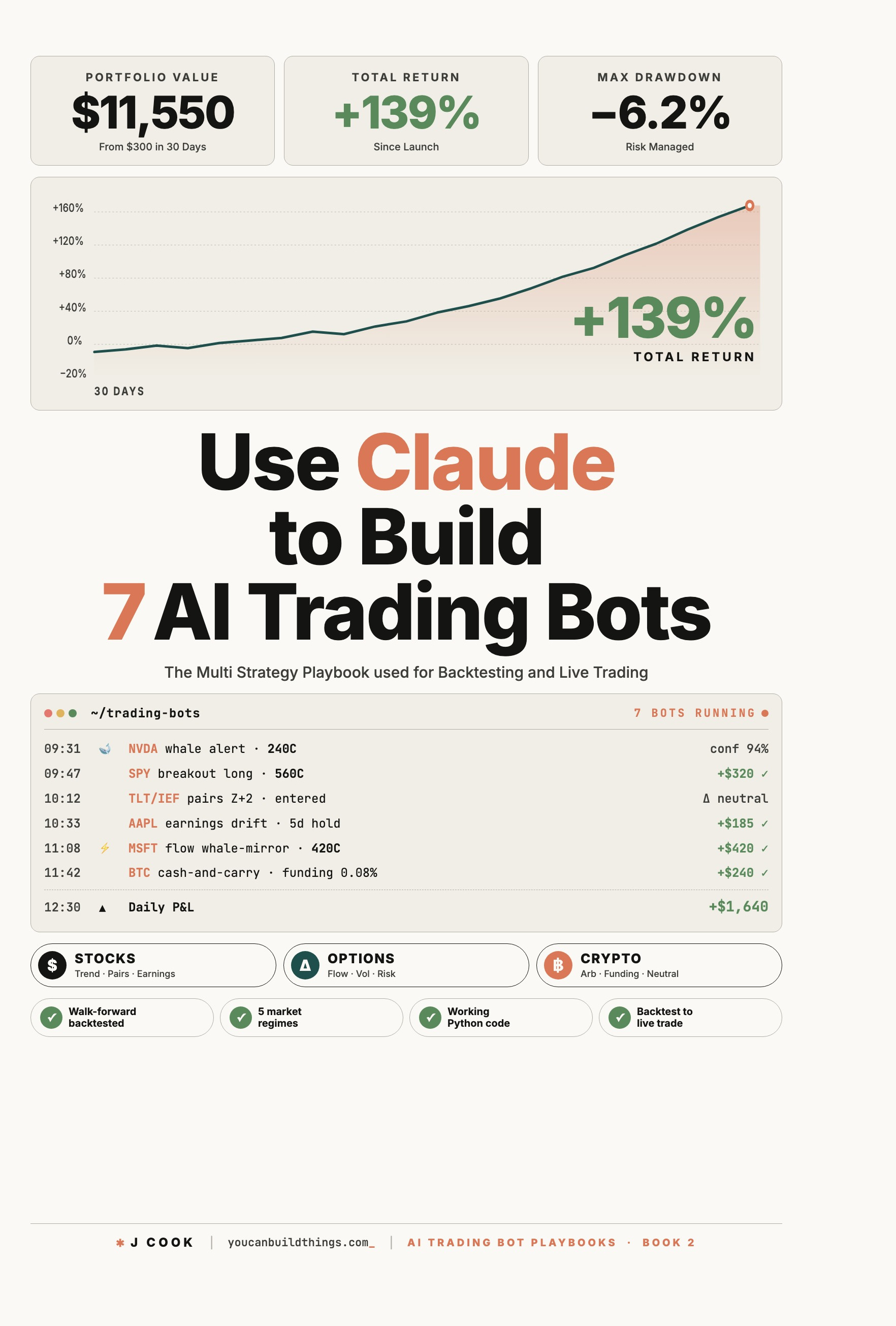
Use Claude to Build 7 AI Trading Bots
Stocks, Options, Crypto. The Multi-Strategy Playbook for Backtest to Live Trade
Summary:
- Cointegration pairs trading Python starts with the right test: Engle-Granger, not correlation. Two random walks that wiggle together are not tradeable; two prices linked by a stationary spread are.
- Run
statsmodels.tsa.stattools.cointon candidate pairs. Trade only when the p-value is below 0.05 on a rolling 252-day window.- Enter at Z-score ±2.0, exit when Z crosses zero or the 20-day time-stop fires. Skip new entries while VIX is above 30.
- Size both legs by the regression hedge ratio, not equal dollars. The hedge is the entire reason this is a real pairs trade.
Most cointegration pairs trading Python tutorials end at “the test passed, here’s the chart.” The bot is missing. The hedge-ratio sizing is missing. The time-stop is missing. The reader builds something on correlation, loses money on uncorrelated random walks, and concludes the math does not work. The math works. The implementation is what is usually broken.
Why does cointegration beat correlation for pairs trading?
Cointegration tests the actual structural relationship between two price levels; correlation tests whether their daily returns track. Two random walks can have correlated daily returns by chance. Their prices have no economic reason to converge. Trading their spread on a Z-score signal is gambling on revert-to-mean for series that do not revert.
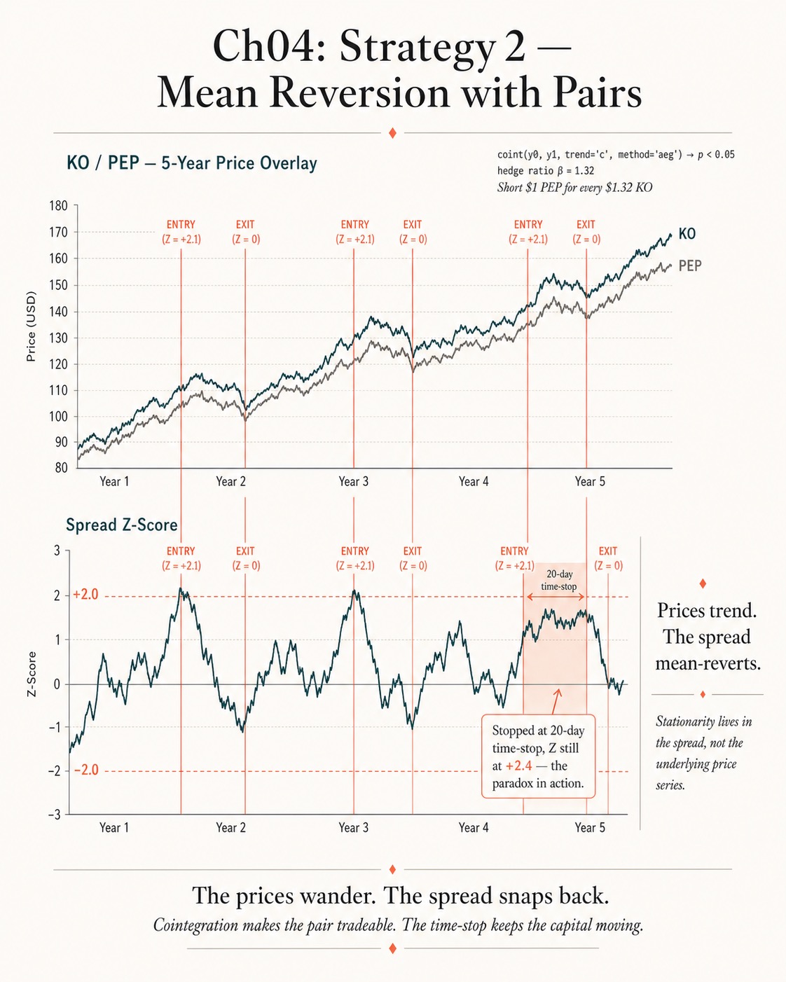
KO and PEP are economically tied. Both sell sugary brown drinks to roughly the same customers in roughly the same channels. When their relative price stretches, the spread tends to pull back, because the underlying businesses are still tied. That is cointegration: two non-stationary series linked by a stationary spread. It is what makes pairs trading a real edge instead of an artifact.
The correlation-only approach is the most common reason retail pairs bots lose money. The fix is to never enter a trade on correlation alone. Run the cointegration test. Trust the p-value. Skip pairs that fail.
How do I run the Engle-Granger test in Python?
You use statsmodels.tsa.stattools.coint. One function call, one threshold check (statsmodels 0.14.6 docs):
# pip install statsmodels
from statsmodels.tsa.stattools import coint

# Function signature (statsmodels 0.14.6):
# coint(y0, y1, trend='c', method='aeg', maxlag=None, autolag='aic', return_results=None)

# y0 and y1 are pandas Series of daily closes for two assets,
# aligned to the same date index (e.g. KO and PEP)
t_stat, p_value, crit_values = coint(y0, y1, trend='c', method='aeg')

if p_value < 0.05:
    print("cointegrated; pair is tradeable")
The docs are explicit about what passes and what does not:
“The Null hypothesis is that there is no cointegration, the alternative hypothesis is that there is cointegrating relationship. If the pvalue is small, below a critical size, then we can reject the hypothesis that there is no cointegrating relationship.”
P-value below 0.05 means you reject the null and the pair is tradeable. P-value above 0.05 is statistical noise: two random walks that happened to wiggle in similar ways. Skip those.
One critical detail no tutorial puts in the headline: cointegration drifts. A pair that was cointegrated last year can lose the property this year because something fundamental changed. The standard practice is to re-run the test every 60 trading days on the rolling window, and drop pairs that fail. Never assume a pair is permanently cointegrated; verify, trade, re-verify, adjust.
How do I compute the Z-score and pick entries?
Z-score normalizes the spread to standard-deviation units. Above +2.0, the rich asset is overpriced; short the rich one and long the cheap one. Below -2.0, the inverse. When Z crosses zero, close.
import numpy as np
import pandas as pd

def hedge_ratio(y0: pd.Series, y1: pd.Series) -> float:
    """OLS slope from regressing y1 on y0. The hedge ratio sizes both legs."""
    return float(np.polyfit(y0, y1, 1)[0])

def zscore_today(y0: pd.Series, y1: pd.Series, hedge: float, lookback: int = 60) -> float:
    spread = y1 - hedge * y0
    rolling_mean = spread.rolling(lookback).mean()
    rolling_std = spread.rolling(lookback).std()
    return float((spread.iloc[-1] - rolling_mean.iloc[-1]) / rolling_std.iloc[-1])

# Entry rule
def entry_signal(z: float) -> str | None:
    if z > 2.0:
        return "short_y1_long_y0"
    if z < -2.0:
        return "long_y1_short_y0"
    return None
Why ±2.0 and not ±1.5 or ±2.5? Convention. Two standard deviations are roughly the 95th percentile of a normal distribution; the spread is rarely there for long. Tighter thresholds trigger more trades but more false signals. Looser thresholds trigger fewer trades but the spread sometimes blows past 2.5 and stays there for weeks. ±2.0 is the published-literature default and it has held up across five regimes.
The candidate basket to scan first: KO/PEP (consumer staples), XLE/USO (energy), GLD/SLV (precious metals), MSFT/GOOGL (mega-cap tech). These are candidates the test will evaluate, not pre-cointegrated pairs you can trust today. Run the scanner; the famous pair name does not pre-qualify the trade.
How do I size both legs with the hedge ratio?
By the slope of the regression. If np.polyfit returns 1.32 for the regression of PEP on KO, you short 1.32 dollars of PEP for every 1.00 dollar of KO you are long. The dollar P&L on each leg roughly cancels when both move together; you only collect when the spread itself reverts. The whole point of the structure.
Equal-dollar sizing is the most common rookie error. If you long $1,000 of KO and short $1,000 of PEP at a 1.32 hedge ratio, you are net-directional on the pair and you have lost the hedge. The trade now bleeds whenever the broader market drifts in either direction. The pair stops being a pair.
def size_legs(risk_dollars: float, hedge: float, spread_vol: float):
    """Risk dollars are spent on the spread's volatility, not the underlyings'.
    Long leg notional sized first; short leg scaled by hedge ratio."""
    long_notional = risk_dollars / spread_vol
    short_notional = long_notional * hedge
    return long_notional, short_notional
Risk per pair is 0.5 percent of account equity, not 1 percent. Pairs trades are bounded by the time-stop, but the worst case in a 20-day window can still be large if the spread blows out. Half a percent is the right starting point; size up only after a full regime cycle of clean live-paper data.
Why use a time-stop instead of a price-level stop-loss?
Because the math is inverted. In trend following, when a trade goes against you, the edge is gone and you exit. In pairs, when a Z-score that hit +2 is now at +3, the statistical edge is bigger, not smaller. A stop-loss at Z=+3 cuts you out of a higher-edge position than the one you entered.
The fix is two-pronged.
Time-stop, hard. Close the trade after 20 trading days regardless of where the spread is. If a cointegrated spread has not reverted in a month, something has changed about the relationship and the original cointegration assumption may be void. Twenty days is the published-literature default; it is also short enough that a broken pair does not bleed for months.
VIX regime filter. Cointegration breaks down during high-volatility regimes. The 2020 COVID liquidity event broke most pairs for several weeks. The bot sits out when VIX is above 30: no new entries, open positions ride out under the time-stop, resume scanning when VIX drops back below 30 for several consecutive days.
import yfinance as yf

def vix_filter_ok() -> bool:
    """No new entries when VIX is above 30."""
    vix = yf.Ticker("^VIX").history(period="5d")["Close"]
    return float(vix.iloc[-1]) < 30.0

def time_stop_hit(entry_date, today) -> bool:
    """20-trading-day hard exit, applied even if the spread has not reverted."""
    return (today - entry_date).days >= 28  # ~20 trading days
The combination is what saves you. The time-stop bounds individual-trade exposure; the VIX filter bounds systemic exposure. Together, they replace the role a price stop would play in a directional strategy, with the math working in your favor instead of against you.
What broke
Three failure modes hit this strategy in the first month of paper trading.
The scanner returns zero cointegrated pairs. This will happen on certain sector baskets in certain regimes. Your basket of four pairs is too small. Expand to a wider universe (S&P sectors, ETF pairs, large-cap-vs-mid-cap rotations). Twenty pairs scanned to find two tradeable pairs is a normal hit rate. Do not weaken the p-value threshold to fix this. Expand the basket.
The time-stop fires on a trade that is “right around the corner” from reverting. Two days after the time-stop closed your position, the spread reverts to zero and you watch the profit you would have had. Resist widening the time-stop. The 20-day rule protects you from the trade that does not revert in 60 days, and you will hit one of those eventually. The cost is the occasional missed late-revert; the benefit is not holding losers for months.
The VIX filter activates mid-trade. Two reasonable policies, pick one and stick with it. Existing positions ride out under the time-stop, no new entries. Or existing positions close immediately, no new entries. The wrong move is to switch policies mid-backtest or mid-live; that adds randomness to your results and makes them un-attributable.
What should you actually do?
- If you are running a pairs bot today on correlation only → swap the entry condition to
coint(y0, y1).pvalue < 0.05this weekend. It is the single highest-impact change; expect 30 to 50 percent of would-be losers to disappear. - If you have cointegration handled but use equal-dollar sizing → wire the hedge ratio into both legs immediately. The bot is otherwise net-directional and you have no hedge.
- If you have a price-level stop-loss → replace it with the 20-day time-stop. Run a backtest with both versions on the same pairs over the same windows; the time-stop version wins, every time.
- If your bot kept losing in the spring of 2020 → add the VIX > 30 filter. Cointegration breaks during crises; the filter is what keeps the bot quiet through them.
- If the scanner finds zero pairs → expand the basket, do not lower the p-value threshold. A 0.05 floor is the math; it does not bend.
bottom_line
- Correlation is not the test. Cointegration is the test. If you are not running
cointon a rolling window, you are not actually trading pairs. - Equal-dollar sizing kills the hedge. Size both legs by the regression slope or the trade is just two independent bets.
- The time-stop is the discipline. The price-level stop-loss is the math working against you. Pick one; the choice has already been made for you.
Frequently Asked Questions
What is the difference between correlation and cointegration in pairs trading?+
Correlation says two return streams move together day to day. Cointegration says two non-stationary price series are linked by a stationary spread that mean-reverts when stretched. Trading correlated random walks loses money; trading the spread of cointegrated pairs is the actual edge.
How do I size both legs of a pairs trade with the hedge ratio?+
The hedge ratio is the slope of the regression of one series on the other. If KO and PEP regress with slope 1.32, the short leg's notional is 1.32 times the long leg's notional. Equal dollar sizing leaves you net-directional and burns the hedge.
Why use a time-stop instead of a price-level stop-loss in pairs trading?+
Because a Z-score that hit +2 and is now at +3 has a bigger expected pull-back, not a smaller one. A price stop systematically cuts your winners and keeps your losers. The 20-day time-stop bounds exposure with the math working in your favor.